PulseCap: Kernel Module for Capturing Timing of Periodic Signals
Periodic signals, such as PWM, are very common in embedded systems. They control servos, light levels just to name a few. The accurate generation of such signals is crucial to enable a precise control. Typically, this analysis is done with an external oscilloscope and analysis software.
To simplify the work and require less external resources, we have prepared a hardware capture system: pulsecap is a HW module and a kernel driver which captures the timing of digital signals. It is accompanied by a python script for basic visualizations.
Overview
To visualize digital signals, typically an oscilloscope is used which samples the input signal at a constant sample rate and visualizes the results over time. Instead of constant sampling, one could describe any digital signal as a sequence of when rising and falling edges happen. The kernel module pulsecap employs the latter view. It utilizes two hardware timers (32bit at 100MHz) to capture the timing of rising and falling edges. With this, it can measure signals at 10ns accuracy.
The FPGA is configured with two pulsecap timers: pulsecap0 connects to the PMOD pin JC2_P, pulsecap1 connects to LED0. Different configurations require a new FPGA bitstream.
Control
The pulsecap module should be loaded automatically based on the
availability of the hardware timers. To check that the module is loaded
use lsmod and check for pulsecap. If the pulsecap module is not
loaded, insert it manually by:
modprobe pulsecap
The pulsecap model is accessible using kernel’s sysfs subsystem. Its control files are located at (X is an instance number, either 0 or 1):
/sys/class/pulsecap/pulsecapX
Each instance folder contains a control folder with the relevant files:
| Name | Description |
|---|---|
| capture | R/W. Write: start capturing of N (integer) edges. Read: how many edges have been captured. |
| state | R. Read: reports current state (idle,running). |
| max_edges | R. Read: maximum number (integer) of edges that can be captured. |
| edge_data | R. Read: can be read only in idle state. Contains timestamp of captured edges starting with the first rising edge. rising and falling edge timestamps alternate. Each timestamp is a 32bit unsigned integer off a 100Mhz counter. When reaching maximum value, timer rolls over and starts at 0 again. User is responsible to deal with timer roll over. Maximum duration between two edges 232/100.000.000 seconds. |
| cancel | write anything to this file to cancel an ongoing capture. |
Examples
The following example shows some helpful commands for pulsecap
# define PulseCap instance
export PCAP=/sys/class/pulsecap/pulsecap1/control

# get max number of edges
cat $PCAP/max_edges

# get current state
cat $PCAP/state

# start recording 20 edges
echo 20 > $PCAP/capture

# check how many edges have been recorded already
cat $PCAP/capture

# copy data into file
cat $PCAP/edge_data > myFile
Hint: When validating the timing of individual pulses, it is sufficient to capture few edges (e.g. 20). Conversely, in order to get the raw data for analyzing the statistical behavior (e.g. raw data for CDF), capture as many edges as possible to get statistically relevant results.
Viewing Data Captured with PulseCap
To view the data you have captured with PulseCap, use the python
application (edgeutil) that is available in the skeleton repository
for Lab 2 (located in the utils folder). Consult edgeutil help page
to see available options:
cd /path/to/edgeutil
./edgeutil -h
Visualizing Data
Once you capture an edge dump, you can feed it to edgeutil in order to
plot and inspect the captured signal. Note that edgeutil runs on the
development environment, while the raw data is stored locally on the
ZedBoard. Transfer the data from ZedBoard to development environment
using scp.
scp root@10.42.1.1:<pathToFileOnZed> <pathToLocalFile>
Then, start edgeutil to plot and inspect the captured signal. If you have graphical output:
./edgeutil <RAW_EDGE_FILE>
Edgeutil can output to an image file for systems without graphical
output (e.g. WSL). For WSL, place the <IMAGE_FILE> where windows can
read it, e.g. /mnt/C/User/<windows_user_name>/Downloads.
./edgeutil --saveplot <IMAGE_FILE> <RAW_EDGE_FILE>
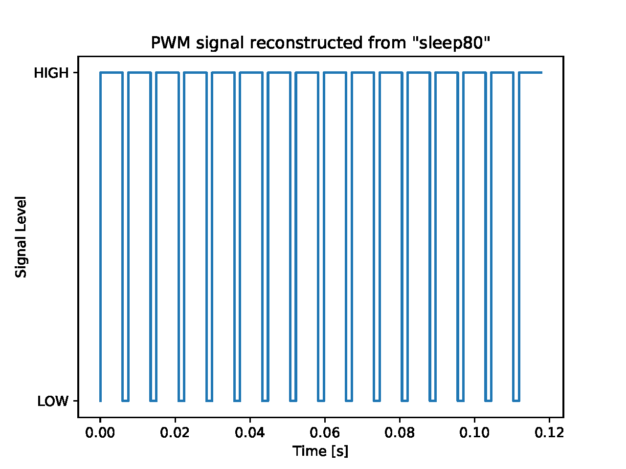
An example visualization of a capture can be seen in Figure 1. You will be able to zoom in and manipulate the capture graph in order to explore the values that you got from the PulseCap module.
Export Data for Post Processing
In order to post process the data (e.g. to calculate CDF) the binary data can be exported into a CSV file. The export automatically takes care of a possible timer roll over during capture (hardware timer is 32bit only) for calculating durations.
To save edge data in a CSV file for posterior processing call:
./edgeutil --output capture.csv raw_edge_file
The saved file is a comma separated file with the format outlined in the table below. All time stamps and durations are in seconds.
| Column | Description |
|---|---|
| 1 | Sample Time |
| 2 | Edge type (0 for RISING, 1 for FALLING) |
| 3 | Duration since last edge of same type (e.g. RISING -> RISING) |
| 4 | Duration since last edge of opposite type (e.g. FALLING -> RISING) |
Make sure to save the exported data with meaningful file names for later analysis.